Linear Regression of multivariate data

In this example, we demonstrate how to use sklearn_xarray classes to solve a simple linear regression problem on synthetic dataset.

This class demonstrates the use of Stacker and Select.

import numpy as np
import xarray as xr
from sklearn.linear_model import LinearRegression
from sklearn.pipeline import make_pipeline, make_union

from sklearn_xarray import Stacker, Select

# Make synthetic data
lat, lon = np.ogrid[-45:45:50j, 0:360:100j]
noise = np.random.randn(lat.shape[0], lon.shape[1])

data_vars = {
    'a': (['lat', 'lon'], np.sin(lat/90 + lon/100)),
    'b': (['lat', 'lon'], np.cos(lat/90 + lon/100)),
    'noise': (['lat', 'lon'], noise)
}

coords = {'lat': lat.ravel(), 'lon': lon.ravel()}
dataset = xr.Dataset(data_vars, coords)

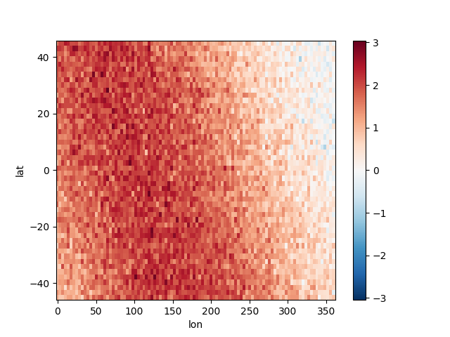
make a simple linear model for the output

\[y = a + .5 b + 1\]

x = dataset[['a', 'b']]
y = dataset.a + dataset.b * .5 + .3 * dataset.noise  + 1

y.plot()

now we want to fit a linear regression model using these data

mod = make_pipeline(
    make_union(
        make_pipeline(Select('a'), Stacker()),
        make_pipeline(Select('b'), Stacker())),
    LinearRegression())

for now we have to use Stacker manually to transform the output data into a 2d array

y_np = Stacker().fit_transform(y)
print(y_np)

Out:

<xarray.DataArray (samples: 5000, features: 1)>
array([[ 1.138895],
       [ 0.799281],
       [ 0.790091],
       ...,
       [-0.134265],
       [ 0.388912],
       [-0.173836]])
Coordinates:
  * samples   (samples) MultiIndex
  - lat       (samples) float64 -45.0 -45.0 -45.0 -45.0 -45.0 -45.0 -45.0 ...
  - lon       (samples) float64 0.0 3.636 7.273 10.91 14.55 18.18 21.82 ...
  * features  (features) int64 1

fit the model

mod.fit(x, y_np)

# print the coefficients
lm = mod.named_steps['linearregression']
coefs = tuple(lm.coef_.flat)
print("The exact regression model is y = 1 + a + .5 b + noise")
print("The estimated coefficients are a: {}, b: {}".format(*coefs))
print("The estimated intercept is {}".format(lm.intercept_[0]))

Out:

The exact regression model is y = 1 + a + .5 b + noise
The estimated coefficients are a: 0.9826705586550489, b: 0.5070234156860342
The estimated intercept is 1.0154227436758414

Total running time of the script: ( 0 minutes 0.584 seconds)